About Level Or Percentage Staking

The blog article “A comparison of level and percentage staking” written by Joseph Buchdahl (@12Xpert) shows the importance of choosing a staking strategy and its infuence on the profit, yield and probability of not making profit, after Monte Carlo simulations of 1000 bets.

This article is very interesting and it is useful to learn more about the influence of the bet size on the results of a positive expected value betting method. The presentation of the results is very clear, so I have used the same format. However, these statistics (yield, profit, probability of not making profit) are not enough to compare different betting strategies. From my point of view, it is always required to know more about the risk assumed, so that the betting method is acceptable from a reward/risk point of view. By doing so, I have found that the “pure” Kelly criterion is not viable when applied to level stakes, and it is also too much risky for percentage stakes. Applying fractional Kelly is a compromise solution that improves the results. Additionally, I have applied Monte Carlo simulations with a number of bets greater than 1000.

Unless offered to play the St. Petersburg lottery (a paradox that consists of a game with theoretical infinite Expected Value although it doesn’t seems worth to play), bettors should always try to maximize the reward / risk ratio. However, a high expected profit implies assuming an always greater than desired risk: “No pain, no gain”. But, at least, bettors can decide which is the value of an acceptable risk and then choose the most appropriate bet size, depending on the expected value, the average odds and the number of bets.

With this article, I would like to show why it is very important to take into account the risk through the maximum drawdown, and I will demonstrate that, at least with WinnerOdds statistics (yield, odds and number of bets), percentage stakes with fractional Kelly criterion it is a much better solution than using level stakes in order to optimize the reward/risk ratio.

Previous results

I have reproduced the same calculations of the mentioned article with @MATLAB (the code can be find at the end of this article), in order to obtain the yield, average and median profit and probability of non-profit, with level stakes and percentage stakes with “pure” Kelly criterion.

Kelly criterion bet size = Bankroll · Expected Value / (Odds-1)

Expected Value = Probability · Odds – 1

There are other staking strategies like the fixed profit bet size, that is also explained in the e-book “How to beat the bookies“, by @Miguel_Figueres., but in this article, I will compare only level and percentage staking.

I extracted some conclusions from reading article about the comparison of level and percentage staking:

• The average yield in case of percentage staking is lower than level staking yield. However, the total amount wagered can be so high, as the bankroll can grow exponentially, that the average profit can reach huge values.
• The average profit with percentage staking with Kelly criterion (bet size as a percentage of the current bankroll) is higher than level staking with the same bet size (in units), due to very high profits with a small probability (asymmetry of the profit distribution)
• The median profit (50% probability of being overcome) of level staking is equal to the  average profit, while the median profit in case of percentage staking is lower than the average profit, also caused by the asymmetry of the profit distribution.
• The time to recover after a loss with a percentage strategy is longer.

However, from my point of view, additional statistics should be taken into account in order to select the best staking strategy. These other variables that can be also taken into account are:

• Bankruptcy risk, maximum drawdown and “resign” probability
• Bet size with fractional Kelly
• Variance and number of bets
• Reward/risk ratio

Bankruptcy risk, maximum drawdown and resign probability

As it is also stated in the article written by Joseph Buchdahl, theoretically, the bankruptcy risk in case of percentage staking with Kelly criterion is null, while the risk of bankruptcy for level stakes with the equivalent bet size can be sometimes important.

This is the bankruptcy probability with level staking (using the bet size in units defined by the Kelly criterion):

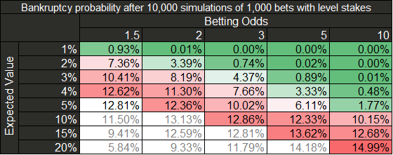
In the results tables, I have used the grey font colour for those “expected value / odds” pairs that are not feasible, as they are really very difficult to achieve and maintain for long series of bets (>1000 bets at least).

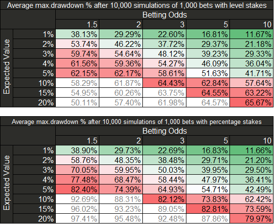
The calculation of the maximum drawdown (maximum difference between the current bankroll and a previous maximum) in units (or money) would not allow the comparison of both staking methods, but we can calculate the maximum drawdown as a loss percentage of a maximum previous bankroll for both staking strategies instead:

Maximum drawdown = Max(1 – Bankroll/Previous maximum bankroll)

The distribution of the maximum drawdown for each staking strategy is show in the following figures:

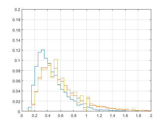
Drawdown distribution for level staking (EV=2%(blue) | 5% (red) | 10% (orange), odds=2.0, bin width=5%)

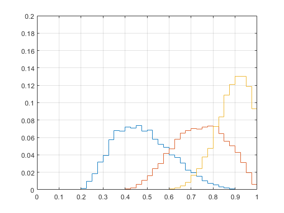
Drawdown distribution for percentage staking (EV=2%(blue) | 5% (red) | 10% (orange), odds=2.0, bin width=2.5%)

It can be observed that the average maximum drawdown percentage with percentage stakes is higher. It is due to the fact that, with level staking, the bet size / bankroll ratio becomes smaller after some growth of the bankroll, while the bet size / bankroll ratio with percentage stakes is constant (and the total amount wagered is much higher). However, the maximum “maximum drawdown” for level stakes can be higher than 100 units, while the maximum “maximum drawdown” for percentage staking is always lower than 100% of the bankroll, as the theoretical bankruptcy risk of the percentage stakes strategy is null. This makes difficutl to compare both strategies.

However, we can consider the probability of “resign”, assuming that a normal bettor would give up betting if the current bankroll becomes lower than 50% of the initial bankroll. On the other side, when the bankroll becomes high enough so that the bettor is “gambling with profit” instead of the initial bankroll, the tolerance to a greater maximum drawdown is increased.

The probability of having at any time a current bankroll lower than 50% of the initial bankroll is higher for percentage stakes when the expected value (and also the bet size) increases:

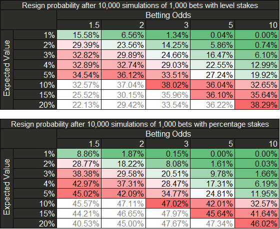
It is evident that, for example, even for a 5% Expected Value method, betting 5% of the bankroll at 2.0 odds is a very risky strategy: Expected maximum drawdowns of 62% and 74%, for level and percentage staking strategies respectively, are not well tolerated by bettors, even taking into account the expected high profits. Using the same example, the resign probability is still 36% and 42%, for level staking and percentage staking respectively.

These results lead to the conclusion that for both staking strategies, using pure Kelly criterion bet size is too risky.

Fractional Kelly strategy

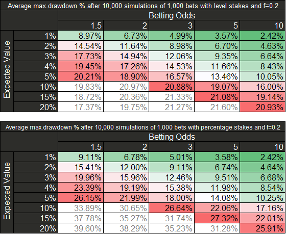
According to the previuous maximum drawdown and resign probability results, it seems reasonable and cautious to use a lower bet size. In WinnerOdds we use a factor f=0.2 times the bet size calculated with the pure Kelly criterion.

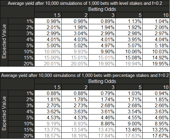
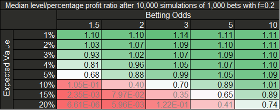
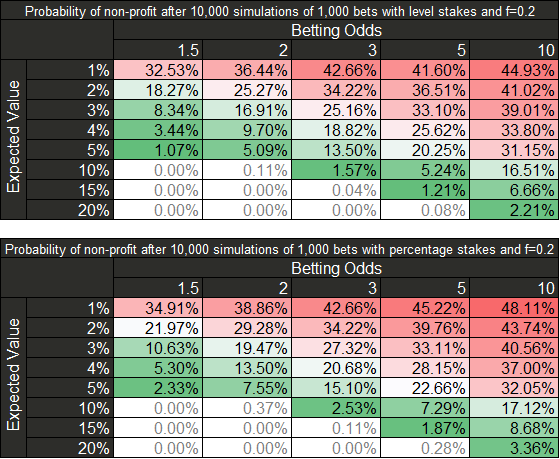
The comparison of the results obtained for both level and percentage fractional Kelly stakes shows that the improvement of the statistics for percentage staking is significant:

• The average yield for level stakes does not vary, while the average yield for percentage stakes becomes greater.

• The median profit ratio between level and percentage staking is closer to 1 in every case

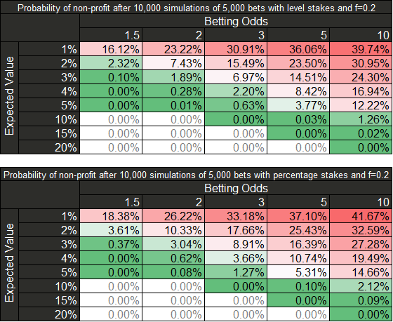
• The probability of not making profit after 1000 bets does not change for level stakes, while it is reduced for percentage stakes with fractional Kelly factor f=0.2.

• The average maximum drawdown is reduced to more acceptable values for both staking strategies.

Variance and number of bets

The variance affects more significantly to the percentage staking, due to the fact that big losses after several consecutive lost bets require longer number of bets to recover. In addition, 1000 bets is a small sample size for any betting strategy. With WinnerOdds, an average user places more than 3000 bets per year.

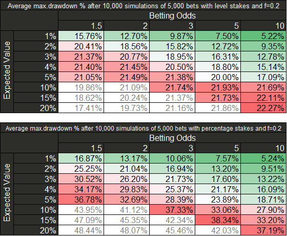
When increasing the number of bets up to 5000, the main differences in the results are:

• Profit increases exponentially for percentage stakes, while it increases linearly for level stakes.
• The yield is not affected by the number of bets
• The median profit ratio between level and percentage staking becomes lower, as the median results for percentage staking increases more than the median with level staking. Only for very low “Expected Value/Odds” pairs, the median of level stakes is higher than the percentage stakes values, and this effect increases slowly with the number of bets.

• The probability of not making profit decreases when the number of bets is higher, although it is always higher for percentage stakes (due to the asymmetry of the profit distribution).

• The average percentage drawdown increases with the number of bets, but is still acceptable.

The opposite conclusions can be obtained for a lower number of bets.

The distribution of the maximum drawdown is more reasonable for Kelly factor f=0.2, taking into account the number of bets.

Drawdown distribution for level staking (EV=2%(blue) | 5% (red) | 10% (orange), odds=2.0, f=0.2, bin width=1%)

Drawdown distribution for percentage staking (EV=2%(blue) | 5% (red) | 10% (orange), odds=2.0, f=0.2, bin width=1%)

Reward/risk ratio

As a bettor, I always try to optimize the reward/risk ratio. Some functions that are used in stock market porfolios comparisons are the Sharpe ratio, the Sterling ratio or the Calmar ratio. In this case, I will use the average profit/average maximum drawdown ratio as an index of the reward/risk value, that is similar to the Sterling ratio.

The results for a bet size with Kelly factir f=0.2 and 5000 bets are:

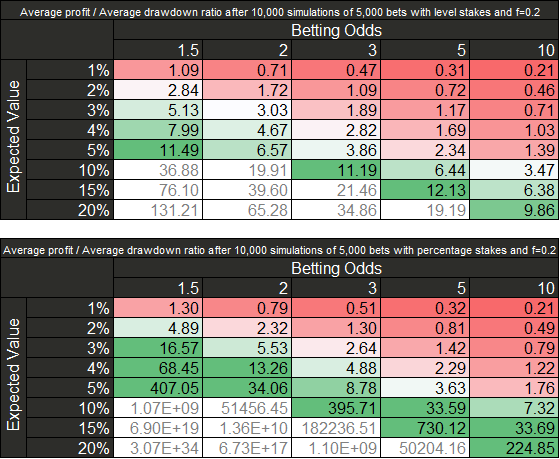
It can be observed that in every case, this ratio is higher for the percentage stakes strategy.

Conclusions

As a result of using a fractional Kelly Strategy, and comparing level and percentage staking strategies, some conclusions can be obtained:

• Both staking strategies have advantages and disadvantages, depending on the odds, Expected Value, and number of bets of the betting method.
• Variance affects more to the percentage staking strategy.
• The asymmetry of the profit distribution makes the median profit to be higher for level stakes than percentage stakes in case of low expected value, higher odds and low number of bets, while the median profit is lower for level stakes than percentage stakes for higher expected value, lower odds and higher number of bets, for a bet size calculated with the same fractional Kelly criterion.
• Using fractional Kelly (f=0.2) makes the yield, maximum drawdown and probability of not making profit of percentage staking become closer to the level staking strategy, although this stats are always better for the last one.
• The average profit/maximum drawdown is always higher for percentage staking strategy, especially for higher Expected Value and lower odds.

This is the summary of the advantages and disadvantages:

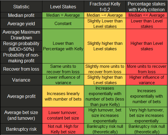
Winnerodds average users results show an average yield of 4%-5%, with average odds around 1.5 and a very large number of bets, higher than 4000 bets per year. These statitics make the percentage stakes strategy with fractional Kelly clearly better than level stakes in this case.

In case of following a betting method that implies relative lower Expected Value, lower number of bets and/or higher odds, it is possible that level staking is a better option.

Level stakes simplicity is also an advantage, especially when the distribution of the betting odds is narrow or the expected value is not known. But in some cases, it can be worth to select the percentage stakes with fractional Kelly strategy in order to optimize the reward/risk ratio as much as possible.

If you like this content, or you have any other idea or strategy, please comment this post! Thank you!

Code

You can change the values and obtain more results, using the following @MATLAB code. Any improvement, suggestion or correction is welcome ☺.
yield = [0.01, 0.02, 0.03, 0.04, 0.05, 0.10, 0.15, 0.20];
odds = [3/2, 2, 3, 5, 10];
betsize = 0.05;
nbets = 1000;
mciter = 10000;
bank_ini = 100;
resign = 0.5;
f_kelly = 1;

% Stats
profit_lvl = zeros(length(yield), length(odds), mciter);
yield_lvl = zeros(length(yield), length(odds), mciter);
mu_lvl = zeros(length(yield), length(odds), mciter);
sigma_lvl = zeros(length(yield), length(odds), mciter);
maxdd_lvl = zeros(length(yield), length(odds), mciter);
maxdd_percentage_lvl = zeros(length(yield), length(odds), mciter);
emaxdd_lvl = zeros(length(yield), length(odds), mciter);
resign_lvl = zeros(length(yield), length(odds), mciter);
bankrupt_lvl = zeros(length(yield), length(odds), mciter);
ROI_lvl = zeros(length(yield), length(odds), mciter);
profit_per = zeros(length(yield), length(odds), mciter);
yield_per = zeros(length(yield), length(odds), mciter);
mu_per = zeros(length(yield), length(odds), mciter);
sigma_per = zeros(length(yield), length(odds), mciter);
maxdd_per = zeros(length(yield), length(odds), mciter);
emaxdd_per = zeros(length(yield), length(odds), mciter);
resign_per = zeros(length(yield), length(odds), mciter);
ROI_per = zeros(length(yield), length(odds), mciter);

for i=1:length(yield)
for j=1:length(odds)
disp([‘Yield=’ num2str(yield(i)) ‘ Odds=’ num2str(odds(j))]);
for k = 1:mciter
prob = (1+yield(i))/odds(j);
T = rand(nbets,1)<prob;
betsize = f_kelly*(prob*odds(j)-1)/(odds(j)-1);
% Level stake stats
res = (T*(odds(j)-1)-(1-T))*betsize*bank_ini;
cumres = [bank_ini; bank_ini+cumsum(res)];
maxres = cummax(cumres);
profit_lvl(i,j,k) = sum(res);
yield_lvl(i,j,k) = profit_lvl(i,j,k)/(nbets*betsize*bank_ini);
mu_lvl(i,j,k) = profit_lvl(i,j,k)/nbets;
sigma_lvl(i,j,k) = std(res,0);
emaxdd_lvl(i,j,k) = emaxdrawdown(mu_lvl(i,j,k), sigma_lvl(i,j,k), nbets);
maxdd_lvl(i,j,k) = max(maxres – cumres);
maxdd_percentage_lvl(i,j,k) = 1-min(cumres./maxres);
if any(cumres<bank_ini*(1-resign))
resign_lvl(i,j,k) = 1;
else
resign_lvl(i,j,k) = 0;
end
if any(cumres<0)
bankrupt_lvl(i,j,k) = 1;
else
bankrupt_lvl(i,j,k) = 0;
end
ROI_lvl(i,j,k) = profit_lvl(i,j,k) / bank_ini;
% Percentage stake stats
res = (T*(odds(j)-1)-(1-T))*betsize;
cumres = cumprod([bank_ini; (1+res)]);
cumbet = betsize*cumres;
cumbet = cumbet(1:end-1);
maxres = cummax(cumres);
profit_per(i,j,k) = cumres(end)-bank_ini;
yield_per(i,j,k) = profit_per(i,j,k)/sum(cumbet);
mu_per(i,j,k) = mean(log(1+res));
sigma_per(i,j,k) = std(log(1+res),1);
emaxdd_per(i,j,k) = emaxdrawdown(mu_per(i,j,k), sigma_per(i,j,k), nbets);
maxdd_per(i,j,k) = 1-min(cumres./maxres);
if any(cumres<bank_ini*(1-resign))
resign_per(i,j,k) = 1;
else
resign_per(i,j,k) = 0;
end
ROI_per(i,j,k) = profit_per(i,j,k) / bank_ini;
end
end
end

t{1,1}=(‘Mean Profit (Lvl)’); disp(t{1,1});
t{1,2}=mean(profit_lvl,3); disp(t{1,2});
t{2,1}=’Mean Profit (Per)’; disp(t{2,1});
t{2,2}=mean(profit_per,3); disp(t{2,2});
t{3,1}=’Mean Yield (Lvl)’; disp(t{3,1});
t{3,2}=mean(yield_lvl,3); disp(t{3,2});
t{4,1}=’Mean Yield (Per)’; disp(t{4,1});
t{4,2}=mean(yield_per,3); disp(t{4,2});
t{5,1}=’Median Profit (Lvl)’; disp(t{5,1});
t{5,2}=median(profit_lvl,3); disp(t{5,2});
t{6,1}=’Median Profit (Per)’; disp(t{6,1});
t{6,2}=median(profit_per,3); disp(t{6,2});
t{7,1}=’Median Lvl / Median Per’; disp(t{7,1});
t{7,2}=median(profit_lvl,3)./median(profit_per,3); disp(t{7,2});
t{8,1}=’Prob of non profit Lvl’; disp(t{8,1});
t{8,2}=mean(profit_lvl<0,3); disp(t{8,2});
t{9,1}=’Prob of non profit Per’; disp(t{9,1});
t{9,2}=mean(profit_per<0,3); disp(t{9,2});
t{10,1}=’Probability of bankruptcy Lvl’; disp(t{10,1});
t{10,2}=mean(bankrupt_lvl,3); disp(t{10,2});
t{11,1}=’Mean of resign Lvl’; disp(t{11,1});
t{11,2}=mean(resign_lvl,3); disp(t{11,2});
t{12,1}=’Mean of resign Per’; disp(t{12,1});
t{12,2}=mean(resign_per,3); disp(t{12,2});
t{13,1}=’Mean of MDD Lvl’; disp(t{13,1});
t{13,2}=mean(maxdd_lvl,3); disp(t{13,2});
t{14,1}=’Mean of MDD % Lvl’; disp(t{14,1});
t{14,2}=mean(maxdd_percentage_lvl,3); disp(t{14,2});
t{15,1}=’Mean of EMDD Lvl’; disp(t{15,1});
t{15,2}=mean(emaxdd_lvl,3); disp(t{15,2});
t{16,1}=’Mean of MDD Per’; disp(t{16,1});
t{16,2}=mean(maxdd_per,3); disp(t{16,2});
t{17,1}=’Mean of EMDD Per’; disp(t{17,1});
t{17,2}=mean(emaxdd_per,3); disp(t{17,2});
t{18,1}=’Mean of Profit/MDD Lvl’; disp(t{18,1});
t{18,2}=mean(profit_lvl,3)./mean(maxdd_lvl,3); disp(t{18,2});
t{19,1}=’Mean of Profit/MDD Per’; disp(t{19,1});
t{19,2}=mean(profit_per,3)./mean(maxdd_per*100,3); disp(t{19,2});

% Histogram plots
histogram(maxdd_percentage_lvl(2,2,:),0:0.05:5,’DisplayStyle’,’stairs’,’Normalization’,’probability’); hold on;
histogram(maxdd_percentage_lvl(5,2,:),0:0.05:5,’DisplayStyle’,’stairs’,’Normalization’,’probability’); hold on;
histogram(maxdd_percentage_lvl(6,2,:),0:0.05:5,’DisplayStyle’,’stairs’,’Normalization’,’probability’); hold off;
axis([0 2 0 0.15]); grid;

histogram(maxdd_per(2,2,:),0:0.05:5,’DisplayStyle’,’stairs’,’Normalization’,’probability’); hold on;
histogram(maxdd_per(5,2,:),0:0.05:5,’DisplayStyle’,’stairs’,’Normalization’,’probability’); hold on;
histogram(maxdd_per(6,2,:),0:0.05:5,’DisplayStyle’,’stairs’,’Normalization’,’probability’); hold off;
axis([0 1 0 0.2]); grid;